A Method for Analysis of Rock Blocks with Complex Arbitrary Geometries

Abstract
The volume, centre of mass, and inertia properties of a block of rock are important physical characteristics when calculating its stability. As a result, civil and geotechnical engineers often need to determine these properties, which are difficult to obtain due to the complex geometry of typical blocks. Currently, the volume of rock blocks with arbitrary geometries are calculated making use of approximations that include, but are not limited to, filling the total volume with tetrahedral blocks and adding up the units; slicing the block in smaller geometrically regular parts; creating profiles of the block, and other analogous methods. Very often, the shapes of the blocks are represented by arbitrary polyhedra with any number of faces and vertices, and a variety of methods can be used to potentially obtain properties of the block from a polyhedron. This work describes a new method to calculate the volume and centre of mass of a block of rock represented by a polyhedron, using vector analysis, analytic geometry, integral calculus, structural geology and rock mechanics theory. Additionally, methods of computational geometry and algorithms are used to demonstrate the processes. The method calculates the volume as a single body improving accuracy that can be affected only by minor irregularities of the rock. It is more effective with the use of computer automation; therefore, technical aspects of the programming procedures will be outlined. The creation of automatic procedures to obtain the results is of great significance to the geotechnical engineering industry, since it will improve the accuracy of results and speed the development of projects. The method is restricted to convex polyhedra, with at least one face exposed to the surface. Keywords: block, rock, polyhedra, arbitrary, geometries, slope, stability
1 - Introduction
The study of the stability of blocks of rock is an important component in the design, construction, and maintenance of roads, dams, buildings, mines, or any project that involves rock as part of the development process. Indeed, engineers have been developing and testing theories to properly analyse the static equilibrium of rocks, which is determined by their physical characteristics and external factors. The volume, density, centre of mass, infilling of the discontinuities, and overall shape of the rock are all aspects that must be considered when determining the safety factor for the stability of potentially unstable blocks of rock. However, because of the natural processes involved in the formation of rocks, the aforementioned theories generally require assumptions to be made, which can affect the calculations and results. One of the critical aspects of these simplifications is related to the calculation of the volume and centre of mass of the blocks, which are usually represented by arbitrary polyhedra. Unlike regular polyhedra, an arbitrary polyhedron is composed of faces of any shape, with many different angles between the edges. These polyhedra can contain forms of great complexity and thus their volume and centre of mass cannot be calculated with a simple mathematical formula.
2 - Methodology
The main objective of this research is to develop a new method to calculate the volume and centre of mass of blocks of rocks with arbitrary complex geometries. To fulfil this objective the following tasks are performed: • Develop a logical sequence of procedures that can be followed for all blocks to obtain the results, independent of their shape or format. • Create the technical foundation for the development of a computer program to calculate the volume and centre of mass of blocks of rock. • Verify the reliability of results based on tests with any type of block. • Investigate already developed code that could be integrated in the final program with little or no modification. • Define the best alternative to acquire data from the field.
3 - Data
Figure 1 shows a typical rock face with many intersecting discontinuities defining rock blocks. Each block is not an isolated body; rather it is usually part of a rock mass and can be delimited by set of planes regardless of 3 minor concavities. The final shape of the block to be analysed depends on the user decision when defining the planes and must be a convex solid.
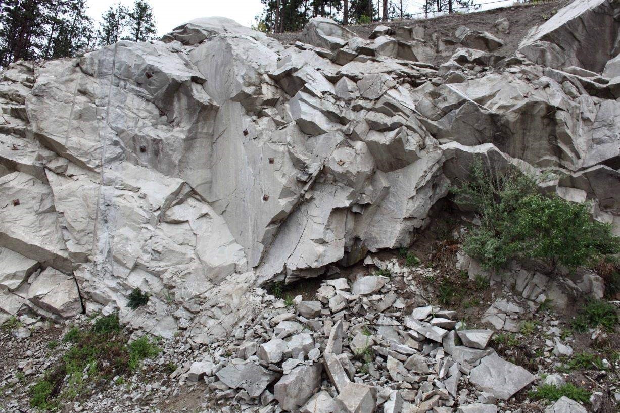
Figure 1. Typical blocky rock mass exposed in a rock face
The initial indispensable information to completely define the block of rock are the orientations of all planes that represent the faces of the block. The advantage of photogrammetry for this definition is that it can produce precise three-dimensional positions of points in the planes in a ground control coordinate system. The process uses a calibrated camera to take pictures of the block of rock from different stations in the ground. The set of pictures is loaded into a software that generates 3D views of the block of rock. In this view it is possible to draw planes that match the faces of the block. The user can read the orientations of planes as dip and dip direction, as well as 3D coordinates of points in the planes, directly from the screen. These parameters must undergo adequate validation to ensure they represent angles and numbers (0˚- 90˚ for dip; 0˚- 360˚ for dip direction; numbers for 3D coordinates). Figure 2 depicts a snapshot of the screen of the 3DM Analyst software used to obtain the block of rock information.
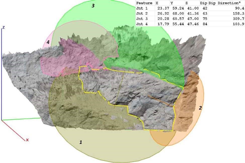
Figure 2. Snapshot of the 3DM Analyst software
3.1 Calculation Procedures
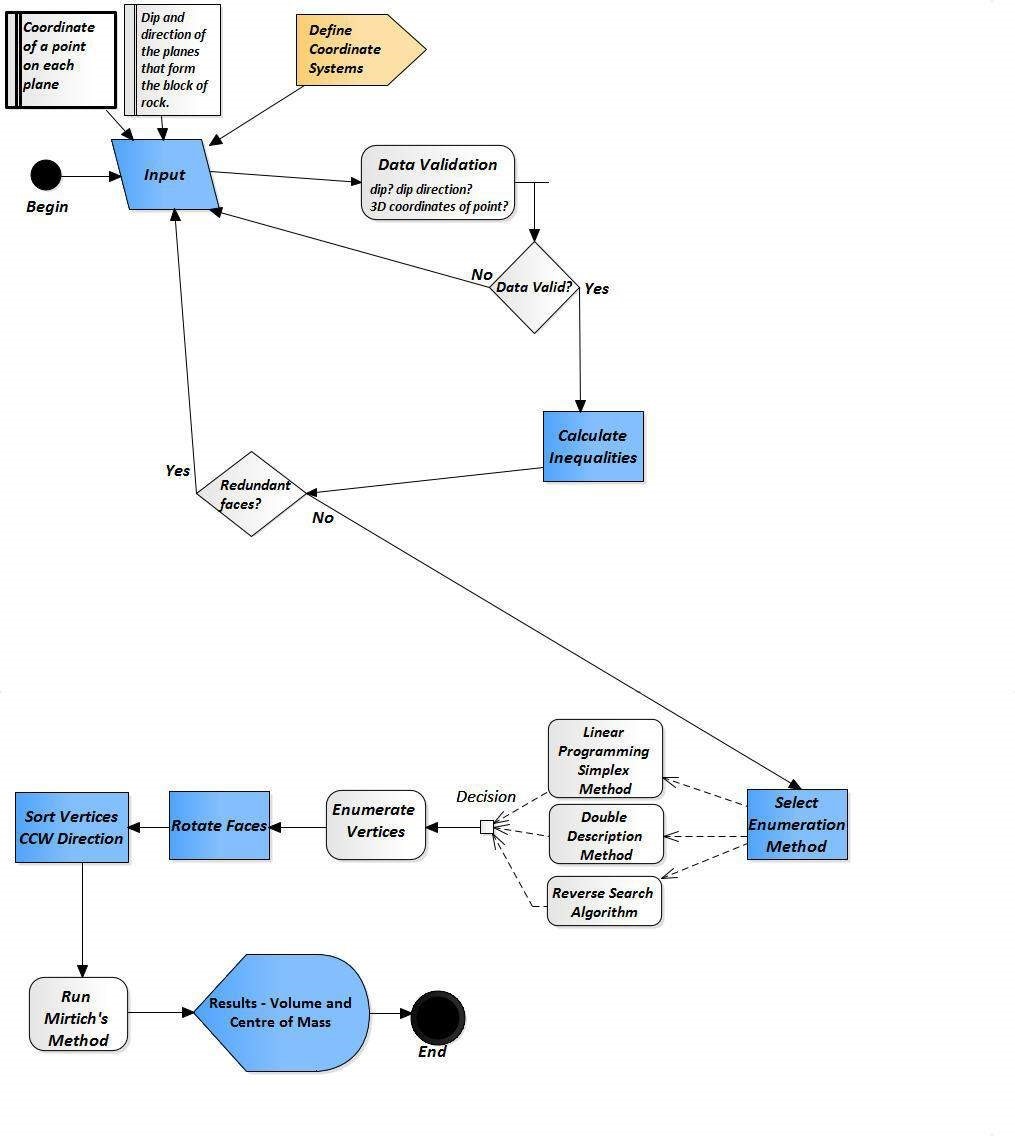
The final calculation of the volume and centre of mass of the block of rock is performed by a computer program developed based on the Method Mirtich described in this paper. The input data to the program are the total number of vertices of the block, the number of faces, and for each face, its number of vertices and an index sorting the vertices of the face in a counter clockwise direction. The starting point to obtain this information uses digital photogrammetry. Once the data is obtained, the equations of the planes that form the block can be calculated using trigonometric relations. The intersection of these planes in space determine the form of the block of rock. Since not all plane intersections are vertices of the block, it is necessary to figure what are the real vertices. The preferable method to obtain the feasible vertices of the block is the Double Description Method (DDM) described below. It is also, possible to obtain the feasible vertices using the Linear Programming Simplex method modified, and the Reverse Search Algorithm that are not described in this text. The DDM have open source computer programs developed for the Linux operating system. When the feasible vertices are obtained, they are distributed in no particular order and the Graham algorithm is used to sort them in a counter clockwise direction on the face. Once this information is available, it is possible to create a file that will be passed to the Mirtich method for the final calculation of the volume and centre of mass. The flow chart in Unified Modelling Language (UML) in Figure 3 outlines the calculation procedures.
3.2 Mass Properties of an Arbitrary Polyhedron – Mirtich Method
The objective of the Mirtich (1996) method is to calculate the mass properties of a rigid body. These properties are the volume V, the centre of mass r, the moments of inertia I, and the products of inertia. Assuming that the body is a polyhedron with uniform density, the method converts the mass integrals into volume 6 integrals. The density of rocks are in the range of 2.5-3.02 g/cm3 but for the same type of rock, the variation usually is between 0.25-0.30 g/cm3. Usually the block of rock in analysis is composed of a single type of rock. Thus, for the purposes of this method the density of the rock can be considered uniform. Classical formulae to calculate moments and products of inertia are the first steps of the method.
- 𝑉= ∫𝑑𝑉 (1)
- 𝑟=𝜌𝑚 〈∫𝑥𝑑𝑉, ∫𝑦𝑑𝑉, ∫𝑧𝑑𝑉〉T (2)
- 𝐼′𝓍𝑥= 𝜌∫〈𝑦2 +𝑧2〉𝑑𝑉 (3)
- 𝐼′𝑦𝑦= 𝜌∫〈𝑧2 +𝑥2〉𝑑𝑉 (4)
- 𝐼′𝑧𝑧= 𝜌∫〈𝑥2 +𝑦2〉𝑑𝑉 (5)
- 𝐼′𝓍𝑦= 𝐼′𝑦𝑥= 𝜌∫𝑥𝑦𝑑𝑉 (6)
- 𝐼′𝑦𝑧= 𝐼′𝑧𝑦= 𝜌∫𝑦𝑧𝑑𝑉 (7)
- 𝐼′𝑧𝓍= 𝐼′𝓍𝑧= 𝜌∫𝑧𝑥𝑑𝑉 (8)
- 𝑉 = ∫𝑉 1 𝑑𝑉 (9)
- 𝑇𝑥 = ∫𝑉 𝑥 𝑑𝑉 (10)
- 𝑇𝑦 = ∫𝑉 𝑦 𝑑𝑉 (11)
- 𝑇𝑧 = ∫𝑉 𝑧 𝑑𝑉 (12)
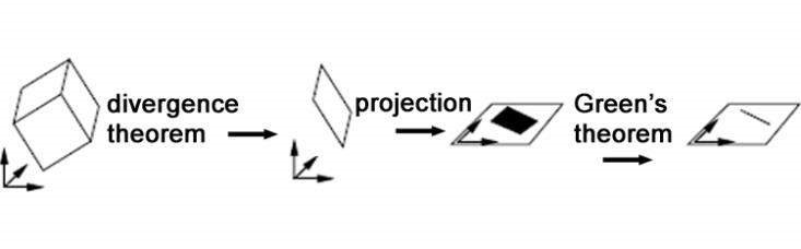
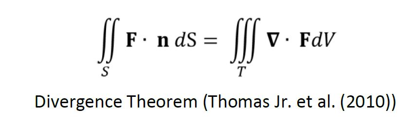
The Mirtich method transforms the formulas to accept the coordinates of the vertices of the block, which will be obtained using the method described in this research. The first step of the Mirtich method uses the divergence theorem, which permits the conversion of a surface integral S over a closed surface into a triple integral over the enclosed region T, or vice-versa.
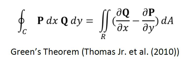
The second step is a preparation to apply Green’s theorem, which is valid over a region on the plane, thus the faces are projected from three-dimensional space onto one of the Cartesian coordinates’ planes. The third step transforms the integrals from the planar region to a linear integral around the edges of every face of the polyhedron. The positive direction, as defined by Green’s theorem, is counter-clockwise. After all conversions of the equations have been made, the integral formulas are obtained in terms of the coordinates of the projected vertices. Figure 5 represents a face of the polyhedron projected on the α-β plane.
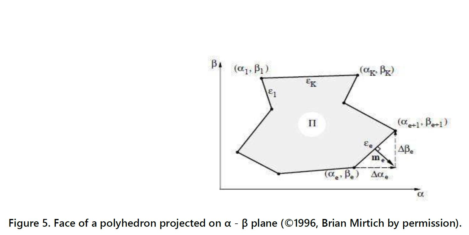
In Figure 5, α and β are the vertex coordinates in the plane αβ, e is the vertex index, k is the number of vertices of the face, and Δ𝛼𝑒 and Δ𝛽𝑒 are the hypotenuses formed by the normal to the edge and the adjacent vertices. The purpose of the method is to calculate simple linear integrals, combine them, and then propagate the results back to obtain the results of the initial integrals.
3.3 Calculation of the Equations of the Planes that Represent the Faces of the Block
Once the dip (𝛷), dip direction (𝜃), and the coordinates x0, y0, z0 of one point (P0) on the geologic discontinuity plane are obtained, the equation of that plane (Equation 13) is calculated using trigonometric relations. 𝐴𝑥 + 𝐵𝑦 + 𝐶𝑧 = 𝐷 (13) The equation depends on the coordinate system defined. When axis x points east, y points north and z points up, the components A, B, and C of the normal vector n to the plane are (Goodman et al., 1985): 𝐴 = sin 𝛷 ⋅ sin𝜃 (14) 𝐵 = sin 𝛷 ⋅ cos 𝜃 (15) 𝐶 = cos 𝛷 (16) The vector normal to the plane is 𝒏 = 𝐴𝐢 + 𝐵𝐣 + 𝐶𝐤 (17) The plane is the set of all points P(x,y,z) and is orthogonal to n. Therefore, the dot product nis equal to zero, and the equation of the plane is calculated: (𝐴𝐢 + 𝐵𝐣 + 𝐶𝐤) ⋅ [(𝑥 − 𝑥0)𝒊 + (𝑦 − 𝑦0)𝒋 + (𝑧 − 𝑧0)𝒌] = 0 (18) (sin𝜙 ⋅ sin 𝜃) (𝑥 − 𝑥0) + (sin 𝛷 ⋅ cos 𝜃) (𝑦 − 𝑦0) + cos 𝛷 (𝑧 − 𝑧0) = 0 (19) Thus, in order to determine the equations of the planes that represent the faces of a block of rock all that is required are the dip and dip direction of the discontinuities that delimit the block and the coordinates of 9 one point on each plane. The number of intersections that the planes create with each other in 3D space can be obtained using Equation 20, where Int is the number of intersections, np is the number of planes and s is the size; which is equal to three because at least three planes are required to create a point intersection. (20) Therefore, combining the plane equations in groups of three will define 3x3 matrices. If each group of matrices has a unique solution, this solution defines a vertex coordinate. A subset of the solutions defines the coordinates that form the block of rock. For example, given the equations of planes 1, 2, and 3, a matrix is formed as follows: Plane1 𝐴1𝑥 + 𝐵1𝑦 + 𝐶1𝑧 = 𝐷1 Plane2 𝐴2𝑥 + 𝐵2𝑦 + 𝐶2𝑧 = 𝐷2 Plane 3 𝐴3𝑥 + 𝐵3𝑦 + 𝐶3𝑧 = 𝐷3 If the determinant , the system has a unique solution and the planes intersect at a point.
4 - Results
4.1 Feasibility of Vertices for a Block of Rock
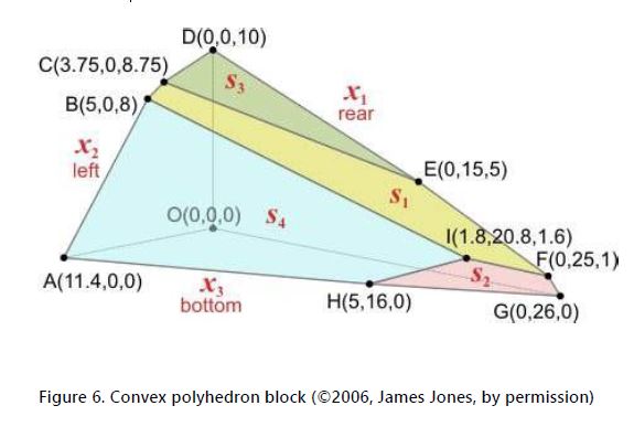
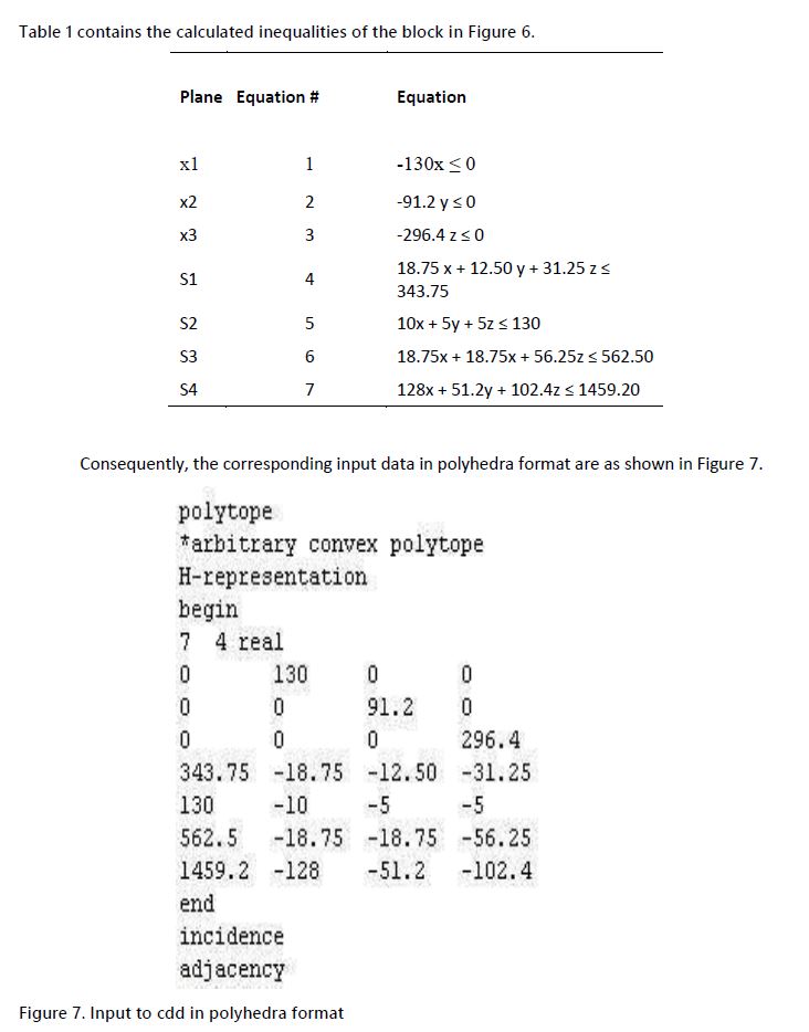
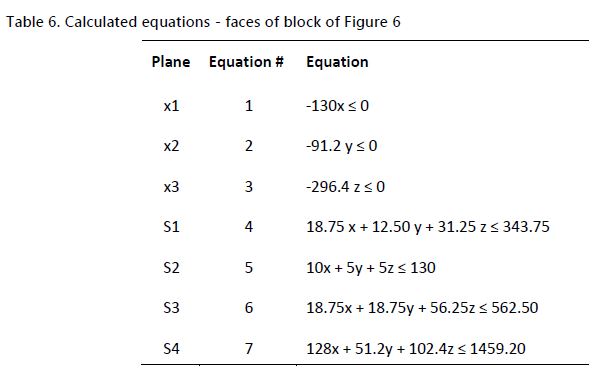
The points generated by the intersecting planes are not all part of the block of rock. For example, the block in Figure 6, which is composed of seven planes, generates a total of 𝐼𝑛𝑡 = 7! / 3!(7-3)! = 35 intersections, as defined by Equation 20. However, only ten of these intersections define the block in this case. These ten points are the feasible points, which are defined as the points at which the vertices of the actual block are located. The concept of a feasible point in a polyhedron is linked to the solutions of a matrix, where the terms of the inequalities that represent the planes of the polyhedron are the rows of the matrix. Using the Gauss Jordan elimination and setting the variables that are not part of the identity sub matrix equal to zero, the remaining variables can be determined, creating a basic solution for the system. If 10 all the variables are non-negative, this is a basic feasible solution that corresponds to the vertices of the polyhedron.
4.2 Identification of the Feasible Points on the Block
The equations of the planes that define the block of rock can be interpreted as inequalities representing hyper-planes. These hyper-planes delimit half-spaces, and their assemblage in space give form to a polyhedron that represents the block of rock. Fukuda (1996) used the Double Description Method invented by Motzin (1953) to obtain the solution of general finite systems of linear inequalities. It was published in the “Contributions to the Theory of Games” in 1950. It is based on the fact that two matrices A and R describe the same object when the following conditions are met: Ax ≥ 0 if and only if x = R λ for some λ ≥ 0 The implementation of this method permits the enumeration of all extreme rays of a general polyhedron in Rd. Professor Fukuda also wrote a program, called cdd, which is available as open source software and can be downloaded from http://www.inf.ethz.ch/personal/fukudak/cdd_home/ and permits the determination of the vertices and the faces that they belong to.
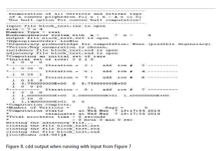
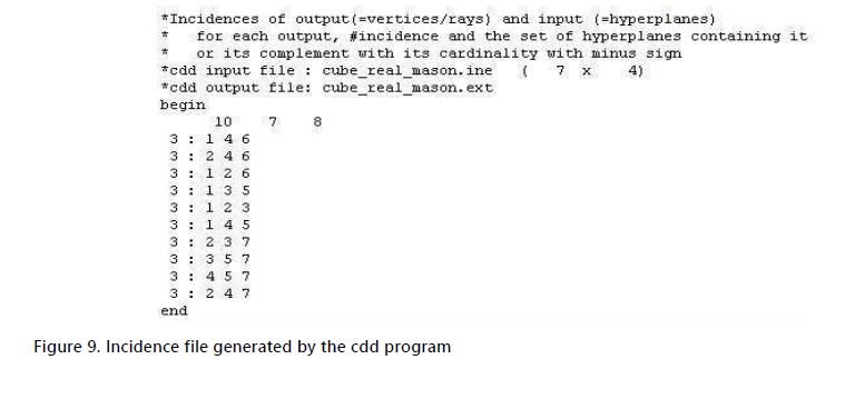
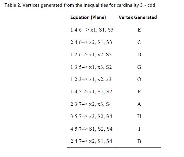
The cdd program output in figure 8 shows the coordinates of the vertices containing the number 1 in the beginning of the line, indicating that it is a valid vertex. The number and coordinates of the vertices of the block perfectly match the ones used to calculate the hyper-planes inequalities. When the number 0 starts the line, it represents a ray. In the case of a block of rock, this is an indication that there is an error in the input data. Additionally, the incidence file generated on Figure 9 provides information that allows the deduction of which face each vertex belongs to.
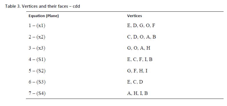
The word begin denotes the start of the output information. The first line after the word begin is the number of outputs. In this case, 10 represent the number of vertices. The second number, 7, is the number m of inequalities (faces) in the input file. The third number is usually m+1, but it will be m when the input linear inequality system is homogeneous. Any line will include the number of inequalities (generally, this number is 3) and their order as defined in the input file. In the case above, inequalities of order 1, 4, and 6 will generate one vertex, 2, 4, and 6 will generate another one, and so on. Using this information, Table 2 can be created, where the planes that intersect to create the vertices are obtained. Consequently, the vertices that are part of each face can be easily determined, and are depicted in Table 3.
4.3 Sorting the Vertices of a Finite Convex Planar Set in the Counter Clockwise Direction
To calculate the volume and centre of mass of an arbitrary block, the Mirtich method requires the coordinates of the vertices on the face sorted in the counter-clockwise direction. After the execution of the Double Description method, the faces and their respective vertices are obtained in no particular order. Consequently, it is necessary to sort the vertices on each face in order to match the required format. Graham (1972) developed an algorithm to find the convex hull from a finite set of points on the plane, which represents the vertices of the faces of the polyhedron. Figure 10 depicts the Graham scan around a set of points.
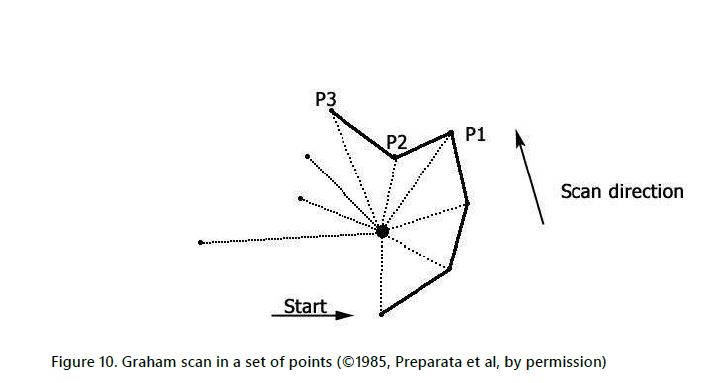
When the initial point is reached, the scan terminates the output and the set of points is sorted in the counter-clockwise direction.
4.4 Running the Graham Algorithm
The input to the Graham algorithm is an unsorted set of points on the plane. The output of the Double Description methods are sets of 3D points, so they cannot be directly used in the Graham algorithm. Thus, the face needs to be rotated around one of the axes to make it parallel to a Cartesian plane. As a result, one of the coordinates will be constant, and the remaining two can be used as inputs to the algorithm. It is important to note that the Graham algorithm will be used only to determine the order of the points on the face. Therefore, after the rotation this order will be obtained corresponding to the existing coordinates before the rotation. Multiplying the coordinates (x, y, z) of all corners of a face as a column vector by the matrix M in Equation 21, the calculated coordinates will be the corners of the face parallel to the x-y plane. The choice of the x-y plane is arbitrary because making the faces parallel to the y-z or x-z planes will produce identical results when the Graham algorithm procedure is applied.
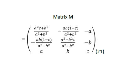
Variables a, b and c are the terms of the unit vector that defines the face from Table 6. The rotated coordinates in the blue rows does not contain the z coordinate since they are constant for each vertex, and are not necessary for the algorithm. There is no need to rotate face x3 since its normal vector is (0, 0, 1). Multiplying the coordinates of the remaining faces by the matrix M causes rotation of the faces, and produces the coordinates in the blue rows of table 7. When the face is already parallel to the x-y Cartesian plane, or in other words, when its normal vector is (0, 0, 1) or (0, 0, -1) a rotation is not necessary and the face’s initial x and y coordinates can be used. Additionally, in cases when the face normal vector is close to (0, 0, 1) or (0, 0, -1) a tolerance must be established to prevent large errors, because some denominators in the matrix are a2 + b2. Since the objective is only to sort the vertices, the results will not be affected.
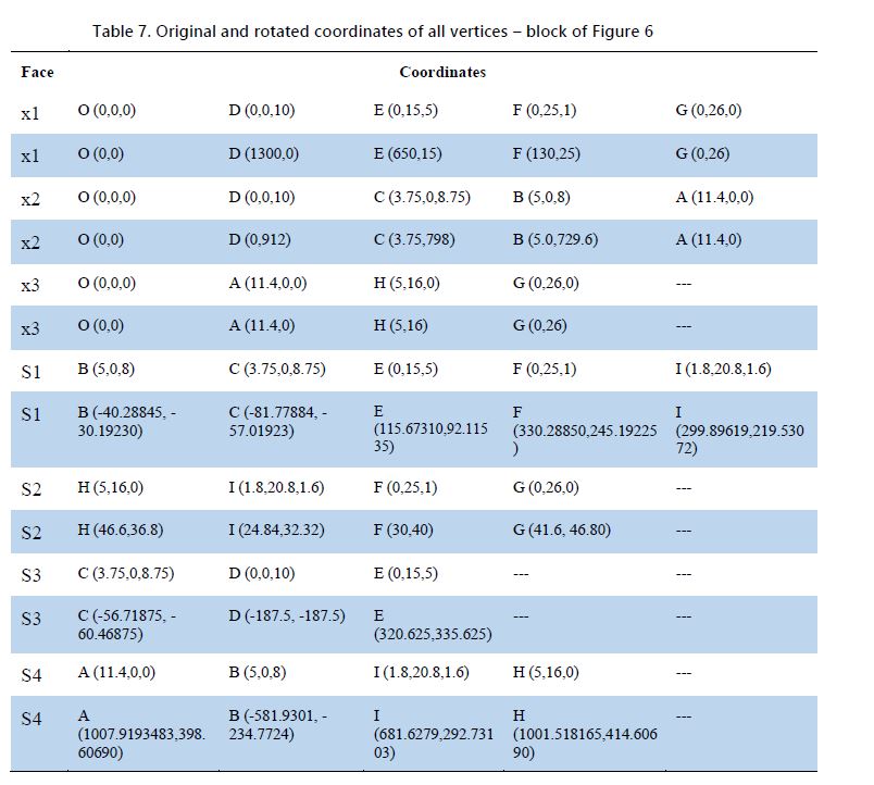
An open source code that implements the Graham algorithm has been modified to fulfil the requirements of this work. Running the Graham algorithm software to the x and y coordinates of each point returns them sorted in a counter-clockwise direction on the face. For example, for face S1, the inputs to the program are the number of vertices (5) of the face, and the rotated x and y coordinates: -40.28845 -30.19230 -81.77884 -57.01923 115.67310 92.11535 330.28850 245.19225 299.89619 219.53072 Figure 11 depicts the input and output of the program.
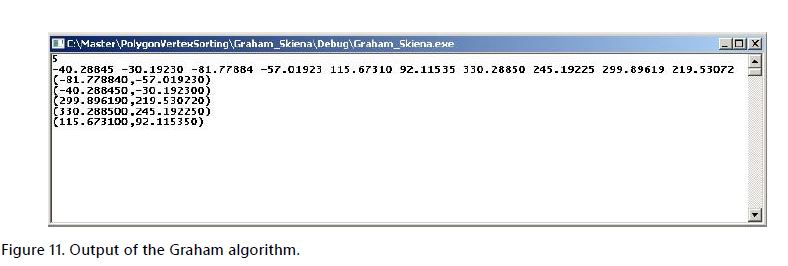
This corresponds correctly to the counter-clockwise direction order of the points C, B, I, F, E on face S1. Likewise, all other faces can have their vertices sorted, and the original corresponding 3D coordinates can be used as input to the Mirtich method, completing the procedure.
5 - Executing the Mirtich method
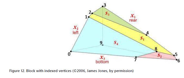
The final step for calculating the volume and centre of mass of the block is to execute the Mirtich method running a program that was developed based on Mirtich’s pseudo code. The input of the program is a data file containing the number of faces, their coordinates, and the number of vertices per face indexed in counter-clockwise direction. To create the data file, the first step is to assign an arbitrary index to each vertex of the block, which ranges from 0 to n-1, where n is the number of vertices. The output of Graham algorithm defines the vertices’ order on each face. For example, face S1 generates the order 1 8 5 4 2. It corresponds to the order obtained from Figure 11, after correlating them with the original coordinates before the rotation. Figure 12 depicts the block with the indexed vertices.
The program automatically identifies the data file structure, which is depicted in Figure 13 for the block of Figure 12. The included descriptions are for clarification only, and are not accepted by the program.
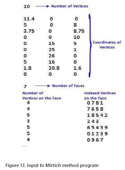
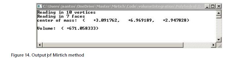
Figure 14 depicts the output of the program, showing the volume and centre of mass of the block in Figure 12.
Conclusions
The main contribution of this research is the development of a method to calculate the volume and centre of mass of blocks of rock with convex arbitrary geometries. The volume and centre of mass of the block of rock is required when calculating its stability and the volume is important when budgeting excavations in large construction projects such as railroads, highways, dams and bridges. The cost to excavate rock is usually paid in terms of volume and the volume is measured in situ. The current methods of investigation to calculate the volume, among others, include drilling, excavation of test pits, or seismic measurements, all of which require the application of significant amount of resources. The availability of a fast and accurate low-cost method to calculate the volume of the arbitrary shaped block would be a significant benefit to such projects, making them more time and cost effective. The method developed in this research requires only the measurements of the orientations of the planes that form the block of rock and the coordinates of one point on each plane. These procedures are fast and can be performed in the field or using digital techniques. However, the use of the method requires computer automation since the calculations involve multiple mathematical techniques, making the calculations impractical without specialized software. The complexity of the calculations arises from the fact that there is no regular geometric form to be used as a template. Consequently, a polyhedron with any number of faces, edges, and vertices is used as a physical representation of the block. This research revealed the technical aspects to confront these problems, indicating solutions for the calculations and a logical procedure for the development of the software. All steps to obtain the solution have been defined, starting with the data collection in the field, the necessary transformation to input into the software and the validation of the data. Once the geologic information is input to the system, the software generates the data transformations and validation, and the output is available almost instantaneously. Depending on the measurement method or the operator, the orientation of the planes that form the block can present small differences. In this context, the software can make several calculations with different data, and the results are easily compared and adjusted. Thus, the accuracy of the results is only dependent on the quality of the input data, since the internal calculations performed by the software are precise. Some code has been already developed, and open source programs are available to be included as is or with minor modifications. Most of these programs were developed as ANSI C standard code that makes it possible to integrate them in the Microsoft Windows operating system, even if developed for the Linux environment. The user interface is generally the quickest part to design, develop, and test, while the core of programming logic usually requires much more effort. Since most of the complex parts have already been developed and tested, future work using this method will provide benefits in terms of cost and reliability.
Acknowledgement
I thank Professor James Jones from the Richland Community College - Illinois – USA for his invaluable help to my understanding of Linear Programming in three dimensions. I must also acknowledge Dr. John Lloyd, Research Engineer, CS, Electrical, and Computer Engineering of UBC, for his help in the search for the best programs to calculate convex hulls and to obtain the right information in computational geometry. I thank Professor David Avis of the School of Computer Science of McGill University for his help with the configuration and use of programs cdd and lrs. Very special thanks go to Dr. Wayne Broughton, Associate Professor of Mathematics at UBCO for providing me the first directions on how to solve the complex problems behind this work.
References
Alexandrov, A.D. 2005. Convex Polyhedra. Springer-Verlag Berlin Heidelberg New York.
Avis, D. and Fukuda, K. 1992. A pivoting algorithm for convex hulls and vertex enumeration of arrangements and polyhedra. Discrete and Computational Geometry, 8: 295-313.
Avis, D. 2000. A revised implementation of the reverse search vertex enumeration algorithm. In Polytopes – Combinatorics and Computation. Edited by Kalai, G. and Ziegler, G., Published by Birkhauser Basel, 29: 177-198.
Avis, D., Fukuda, K., and Picozzi, S. 2002. On canonical representations of convex polyhedra. In Proceedings of the First International Congress of Mathematical Software, p. 350-360, Beijing, China, 17-19 August 2002.
Bland, R. 1977. New finite pivoting rules for the simplex method. Mathematics of Operations Research, 2(2): 103-108.
Birch, J.S. 2006. Using 3DM Analyst mine mapping suite for rock face characterisation. In Proceedings of Laser and Photogrammetric Methods for Rock Face Characterization. Edited by F. Tonon and J. Kottenstette, Golden, USA.
Cromwell, P. 1999. Polyhedra. Cambridge University Press, 1st edition.
Coxeter, H. 1973. Regular Polytopes, 3rd edition, Dover Publications, Inc., New York.
Dantzig, G. and Thapa, M. 1997. Linear Programming vol 1,2, Springer Series in Operations Research - Springer-Verlag, New York.
Dyer, M.E., and Proll, L.G. 1977. An algorithm for determining all extreme points of a convex polytope, Mathematical Programming 12:81-96 – North-Holland Publishing Company.
Elmouttie, M., Poropat, G., and Krähenbühl, G. 2010. Polyhedral modelling of rock mass structure. International Journal of Rock Mechanics & Mining Sciences 47: 544-552.
Fukuda, K., and Prodon, A. 1996. Double description method revisited. Combinatorics and Computer Science, 1120: 91-111.
Fukuda, K. 1999. cddlib Reference Manual, Institute for Operations Research and Institute of Theoretical Computer Science – Zurich ,Switzerland. ftp://ftp.ifor.math.ethz.ch/pub/fukuda/cdd/cddlibman/cddlibman.html [cited July 2014].
Fukuda, K. 2004. Frequently asked questions in polyhedral computation, Swiss Federal Institute of Technology - http://www.cs.mcgill.ca/~fukuda/soft/polyfaq/polyfaq.html [cited July 2014].
Fukuda, K. 2011 – Institute for Operations Research – Swiss Federal Institute of Technology Zurich, https://www.ifor.math.ethz.ch/teaching/lectures/poly_comp_ss11/lecture9 [cited July 2014]
Fukuda, K. 2014. cdd and cddplus homepage. www.inf.ethz.ch/personal/fukudak/cdd_home/index.html [Accessed July 2014]
Goodman, R., and Shi, G. 1985, Block Theory and Its Application to Rock Engineering, Prentice-Hall, New Jersey.
Graham, R. 1972. An efficient algorithm for determining the convex hull of a finite planar set. Information Processing Letters 1: 132-133. North-Holland Publishing Company.
Huang, T., Chen, J., and Chang, C. 2003. Stability analysis of rock slopes using Block Theory, Journal of the Chinese Institute of Engineers, 26(3): 353-359.
Hudson, J., and Harrison, J. 2000. Engineering Rock Mechanics- An Introduction to the Principles, Pergamon – Elsevier Science Ltd.
Jafari, A., and Khishvand, M. 2012. An efficient block detection algorithm in 3D-DDA. In Advances in Discontinuous Numerical Methods and Applications in Geomechanics and Geoengineering, Honolulu-USA
Kaibel, V., Metchel, R., Sharir, M., and Ziegler, G. 2006. The simplex algorithm in dimension three, SIAM Journal of Computing, 34(2), 475-497
Mirtich, B. 1996. Impulse-based Dynamic Simulation of Rigid Body Systems. PhD thesis, Computer Science in the Graduate Division, University of California at Berkeley.
Motzkin, T., Raiffa, H., Thompson, G., and Thrall, R. 1950. The Double Description Method. Contributions to the Theory of Games. Princeton University Press.
Preparata, F., and Shamos, M. 1985. Computational Geometry - An Introduction. SpringerVerlag, New York.
Preparata, F., and Muller, D. 1977. Finding the intersection of n half-spaces in time O(n log n) Mathematics for Key Technologies – DFG Research Center, Berlim
Schubert, W., and Potsch, M. 2005. Kinematical analysis of rock blocks supported by 3D imaging – In Proceedings of the 41st Symposium on Rock Mechanics (USRMS): 50 Years of Rock Mechanics - Landmarks and Future Challenges. Golden, Colorado, June 17-21, 2006
Tannant, D.D, Radmanovic, J., and Jiang L. 2006. Digital photogrammetry for surface mining applications. In Proceedings of CIM Mining Conference and Exhibition, Vancouver, 12 p.
Terzer, M. 2009. Large Scale Methods to Enumerate Extreme Rays and Elementary Modes. PhD thesis, Swiss Federal Institute of Technology, Zurich
Thomas, Jr., Weir, M., and Haas, J. 2010. Thomas’ Calculus Early Transcedentals, 12th edition. Addison-Wesley.
USask. 2014. Strike and Dip. http://homepage.usask.ca/~mjr347/prog/geoe118/geoe118.045.html [cited July 2014]
Warburton, P. 1981. Vector stability analysis of an arbitrary polyhedral rock block with any number of free faces. International Journal of Rock Mechanics & Mining Sciences & Geomech. Abstr. 18: 415-427.
Weisstein, E. 1999. Polyhedron. From MathWorld- A Wolfram Web Resource http://mathworld.wolfram.com/Polyhedron.html [cited July 2014]